Introduction to Matlab 1: All in One View

Content from What is MATLAB?

Last updated on 2025-02-18 | Edit this page

Estimated time: 12 minutes

Overview

Questions

What does MATLAB do?
How can MATLAB help my Research?
Is MATLAB the best tool for my Research project?

Objectives

Explain what tasks MATLAB is well suited for
Explain how MATLAB compares to other common tools (Python, R)
Understand the trade-offs of choosing MATLAB as a tool

Introduction

What is MATLAB?

MATLAB is a high-level propriety programming language and interactive environment primarily designed for numerical computing, data analysis, and scientific visualization. It provides a comprehensive suite of tools for tasks such as matrix manipulation, algorithm development, data plotting, and interfacing with other programming languages. Its user-friendly interface and extensive library of functions make it a popular choice among researchers, engineers, and scientists.

Propriety

MATLAB is a propriety language, this means it is owned by a specific company, MathWorks. Therefore it’s source code is not publically available (i.e., it is the opposite of open-source) and the software is licensed for use under specific terms and conditions. There are many pros and cons of working with propriety software.

Discuss pros & cons

Discuss or think about what might be some of the advantages and disadvantages of software being owned by a single company.

Show me the solution

Feature	Proprietary	Open Source
Cost	Individual MATLAB license is £800/year (£59 one time for students)	Nearly always free
Documentation	Single documentation site with everything you need to know	Can be spread around many site, different communities contributing different documentation
Support	Single company to ask support queries and report bugs to	Reliant on a spread out community for support with no single best place to go
Adoption	Typically used in large companies and academia due to cost	Widely adopted across all parts of the community

Why MATLAB?

While many research tools can accomplish tasks similar to MATLAB, understanding MATLAB’s strengths and weaknesses in comparison is important. Two of the main alternative languages you may have heard of are Python and R (r-project). These are often compared because all 3 languages are often used for research.

High-Level and Low-Level

Low-level code languages are closer to the machine’s language, requiring more precise instructions for the computer to understand. They offer greater control over hardware but are more complex to write and debug. High-level code languages are more abstract and human-readable, translating simpler instructions into the complex machine code. They are easier to learn and maintain but may sacrifice some performance efficiency compared to low-level languages.

MATLAB is considered to be on the high-level end of languages, making it relatively easy to read and work with.

Key Points

MATLAB is used in many fields and can be used to analysis, process, model and much more
MATLAB is proprietary which has its own benefits and costs

Content from Matlab Layout

Last updated on 2024-10-29 | Edit this page

Estimated time: 12 minutes

Overview

Questions

What do all the different parts of the MATLAB interface do?
What features are important to get started in MATLAB?

Objectives

Learn to navigate and adjust the MATLAB interface
Understand the difference between the command window and the editor

Introduction

MATLAB as a language is mainly interacted with through the MATLAB application. Before we press on with learning, writing and running MATLAB, this episode will quickly run through the various parts of MATLAB and help you understand where and how you should write MATLAB.

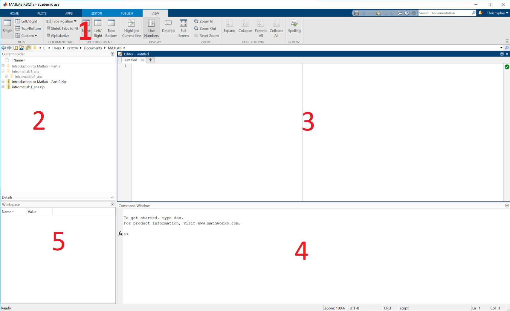
Below is an annotated diagram showing what of the MATLAB application looks like.

A screenshot of the MATLAB application with red numbers annotating the major areas of the application which are detailed in the main body

Layout

Don’t worry if your layout does not match the one in the diagram. The MATLAB application is very customizable and you can drag and drop the various windows around. There are a few preset layouts available in the view tab at the top

Each number on the diagram describes:

Menu Ribbon - This bar functions much like the bars at the top of many Microsoft and Google applications you may be familiar with, it has tabs with different options in. Throughout this course we will be exploring some of these tabs in more detail.
Current Folder - Here you can explore the files on your computer much like the explorer on your computer. The folder currently showing is also known as the ‘Working Directory’ and this is where MATLAB will first search for files.
Editor - This is where you will edit MATLAB code files.
Command Window - One off MATLAB commands can be executed here.
Workspace - You will be able to see any variables that are currently in memory here

If any of this isn’t clear again don’t worry! This course will further explore and clarify all of these tools.

Editor VS Command Window

You can write and run MATLAB code in both the command window and the editor so understanding the purpose (and differences) of each is important.

Command Window	Editor
Quick calculations	Creating and editing persistent scripts
Testing	Reading and using others code
Interactive exploration	Creating functions
Debugging

Challenge 1: Using the command window

What is the output of this command?

13 * 8

Instructor Note

May be worth explaining that * is used for multiplication in many programming languages and / for divide Explain ans = - or at least mention this will be covered later.

Challenge 2: Using the editor

Press ‘New Script’ at the top left and type the following into your editor. Then press ‘Run’ in the EDITOR tab at the top.

b = 136 / 8

What do you have to do in order for the code to run?
What is the output?

Show me the solution

The editor modifies and runs a MATLAB file (m-file), so in order to run what is in the editor you will be required to save the script you have made to a new m-file.
17

As you saw in the challenge above, using the editor requires you to create and save a file with the extension .m. This means that when you next come to do your analysis, processing, etc., you can reopen this file and continue work from it again.

Saving your work

Unlike the editor, any work done in the command window is not saved! This means that if you close MATLAB or your computer this work will be lost. Hence why you should use it only for quick temporary tasks.

Key Points

The MATLAB interface is very customisable, adjust it to suit you
Use the command window for quick tasks like exploring data, testing, etc.
Use the editor for developing code you want to persist between sessions

Content from Creating Variables

Last updated on 2025-02-06 | Edit this page

Estimated time: 12 minutes

Overview

Questions

How can I store and work on data?
What does MATLAB assume about data?
How can I handle data of 2, 3 or more dimensions?

Objectives

Lean about what a variable is and how MATLAB handles variables
Understand how to create variables of various dimensions
Briefly review data types and why they aren’t important in MATLAB

Introduction

When programming there are many occasions where you will want to be able to access some data. For example, you may want to load in a data set from online, load data from an sensor in the field or store the results of a calculation. How we store and refer to data in programming is through the use of variables.

Variables

A variable in MATLAB is made of 2 parts, a name and a value. The name is what we use to refer to a variable and the value is the number, word, or item that is stored in it.

The value of a variable in MATLAB can be many things! Some examples are

Variable Type	Example Value
Integer	1, 2, 3
Double	1.23, 4.56
Character	‘A’, ‘b’, ‘c’
String	“hello”
Matrix	[1 2 3; 4 5 6]
Logical	`true`, `false`

As mentioned in the previous episode MATLAB has a section called the workspace, this is where you can view what Variables are in-memory. The simplest way of creating a variable is with the ‘=’ symbol, for example:

my_variable = 5

will create a variable with the name my_variable and a value of 5.

Memory

MATLAB (like most programming languages), holds variables in-memory. This means they are stored on your computers RAM rather than your hard drive. This allows for fast access and processing, however RAM is wiped when your computer turns off or an application quits so your workspace will be deleted when you close MATLAB or shut off your computer.

Challenge 1: Creating Variables

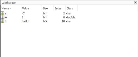
Create a variable called A with a value of 3
Create a variable called B with a value of ‘hello’
Create a variable called a with the value of ‘C’:
Create a variable called C with the value of the variable in A
Customise your workspace and add the extra columns Size, Bytes and Class, this can be done by right clicking the top of the workspace

Show me the solution

A = 3
B = 'hello'
a = 'C'
C = A
Your workspace should look like this! We suggest customising the workspace columns just as an example of what is possible.

Data Types

You may notice in the previous solution there is a type called a ‘double’. MATLAB is whats known as a dynamically typed language, which is also called “duck typing”. This is based off the saying ‘if it walks like a duck and quacks like a duck it’s probably a duck’. In programming terms this means that when you make a variable MATLAB has a look at it and assumes what type it is based on how it looks. Other languages like C++ require you to explicitly tell the program what type every variable is.

For you as a user, this means that you don’t have to really know or pay attention to data types! However it is worth knowing they exist, as if you get more advanced you may want to manipulate them to optimise your algorithms or for some other advanced use cases.

Variable Names

There are several conventions for naming variables, such as camel case, where each word is joined without a space and each new word starts with a capital letter. For example camelCase or analysisResult

Snake case is another common standard, where each word is lower case and separated with underscores, for example snake_case or analysis_results.

Both standards will work well, if you’re working with existing code or on an existing project it is normally best to stick with the convention already in use!

Useful Variable Names

In this lesson we are using variable names without any meaning such as A or B. When programming code it is good practice to use meaningful unique names for your variables.

Dimensions

A lot of data analysis, processing and workflows wont be with single numbers but with large multidimensional datasets. Working with image/video, time series, tables or many other data sources can quickly make your incoming data large in size. Variables in MATLAB can and are very good at storing and working with multidimensional data.

Penny command

Use the penny command in the command window. this command will create an interactive 3D plot of a US penny mold.

How many new variables are there in your work space?
Look at the size column in your workspace, how many dimensions are there in each variable?

Give me a hint

If you double click a variable name in the workspace you can explore it in a spreadsheet style interface called the variable editor.

Show me the solution

There should be 2 new variables in your workspace, P and D. Both have a size of 128x128, this means they have 128 rows and 128 columns and are therefore 2-dimensional matrices.

Dimension Order

In MATLAB learning the order in which dimensions appear is very helpful.

The first dimension is always rows and the second columns. So if you saw a variable with size 5x10, you could picture it looking like a spreadsheet with 5 rows and 10 columns. (This is the opposite if what you would expect from X, Y notation!)

In MATLAB there are names given to different variable shapes:

Dimensions	Name	Description
0D	Scalar	A single value like those created in Challenge #1
1D	Vector	A single row or column
2D	Matrix	Rows and columns, like an Excel spreedsheet or Google sheet
3D+	Array	Rows, columns and pages

An animated GIF showing a vector column, matrix and array being built. It aims to add intuation for the shape of each of these types

Creating Multidimensional Variables

In general when creating multidimensional variables you

use square brackets []
separate columns with a space
separate rows with a semi-colon ;

Here are some examples of creating vector variables:

MATLAB

E = [1 2 3] # 1x3 row vector named E 
F = [4;5;6] # 3x1 column vector called F

Challenge

Create a row vector called G with values 2, 4 & 6
Create a column vector called H with values 1, 3 & 5
Create a 2x2 matrix called I with values 10, 20, 30 & 40.

Show me the solution

G = [2 4 6]
H = [1;3;5]
I = [10 20; 30 40]

Cleaning the Workspace

Finally we will look at how we can remove variables we aren’t using! We do this because as you explore data and test your analysis over time you will get variables you aren’t building cluttering your workspace, this can lead to you either accidently overwriting data or using variables you weren’t intending to.

Clearing all variables

Simply putting clear into your command window will clear all variables

Clear single variable

clear A will clear just the variable called A

Clear command window

After working a while you will have a long history of commands in your command window, you can clear this up by running the clc (command line clear) command.

Callout

You can access commands you have previously typed in the command window by pressing the up arrow on your keyboard. If you type part of a command and press the up arrow, only commands that match the partially completed command will be shown.

Indexing

Colon Notation

MATLAB provides what is called the colon notation which allows us to specify a range of values.

MATLAB

a = 1:10

OUTPUT

a =
     1     2     3     4     5     6     7     8     9    10

a should be 1x10 size, meaning 1 row 10 columns

Steps

You can also specify a step, so the colon notation only makes every nth number

MATLAB

b = 1:2:20

OUTPUT

b =
     1     3     5     7     9    11    13    15    17    19

Steps can also be non-integer values

MATLAB

c = 1:0.1:2

OUTPUT

c =
    1.0000    1.1000    1.2000    1.3000    1.4000    1.5000    1.6000    1.7000    1.8000    1.9000    2.0000

Steps and range end values

When you specify a step that is grater than 1, the last value won’t necessarily be the range end value! Instead it will be the closest value that doesn’t go over the end value and this is why the last value in b is 19 and not 20!

Functions

We can also use functions to create arrays (vectors or matricies). Functions are premade code blocks that serve a commonly wanted functionality.

First we will use one called linspace, which stands for linearly spaced. It creates a vector of linearly spaced numbers, you specify the start, end and how many numbers.

Callout

If you are ever unsure about a function MATLAB has inbuilt help and documentation!

The help command will give a brief text description about the function and how to use it

MATLAB

help linspace

The doc command will give a more detailed description including examples

MATLAB

doc linspace

MATLAB


d = linspace(1,10,5)

OUTPUT


d =
    1.0000    3.2500    5.5000    7.7500   10.0000

Some other useful functions are:

MATLAB

% Rand creates an n-dimensional array of random numberes between 0 and 1.
e = rand(5,1)

% Create 2D matrix of zeros.
f = zeros(2,2)

% Create a 2D matrix of NaN values - NaN means 'Not a Number'
% This is a special and useful term for when a value can't be represented by a number.
g = nan(5,5)

Callout

Here are some common scenarios where NaN may be used:

Mathematical operations that cant be computed (division by 0, root of negative numbers)
No data were recorded, for example an in-field sensor may have lost power

Challenge

Create a vector with numbers 12 to 100 containing every 4th number (steps of 4), called h
Create a matrix of random numbers with 4 rows and 5 columns, call it ii

Show me the solution

h = 12:4:100 or h = linspace(12,100,23)
ii = rand(4,5)

i

i in MATLAB can be used as a variable, but it also has a special meaning as the square root of -1! MATLAB treats j the same way. To avoid confusion it’s often better to use ii and jj instead.

Key Points

Variables are the main way we access and use data in MATLAB
Variables can store many types of data including multidimensional data
Creating multidimensional arrays is done with square brackets

Content from Working with Variables

Last updated on 2025-02-06 | Edit this page

Estimated time: 12 minutes

Overview

Questions

How can I fetch data out of a variable?
How can I change the values of parts of variables?
What are operations?

Objectives

Access MATLAB variables and change them
Use variables to execute mathematical operations and in functions

Introduction

So far we have learnt how to create variables of various sizes with different methods. This episode will now focus on how ways we can use variables.

Now is a good time to clear and clc your workspace and command window!

Extracting Variables

First lets start by making a dummy variable that we can use as our stand-in dataset.

MATLAB

data = 100*rand(6,4);

Subsets

Subsets of values or single values can be extracted from a variable with round brackets ()

For example to take the value on the third row and second column:

MATLAB

data(3,2)

We can use colon notation to extract multiple values as well:

MATLAB

% Extract columns 1, 2, and 3 on row 3
data(3,1:3)

A single colon with no numbers will select all

MATLAB

% Select all rows in the second column
data(:,2)

Some more examples bringing together the tools we’ve seen so far:

MATLAB

% Extract the first 4 rows and all columns and save it in the variable subset1
subset1 = data(1:4,:) 

% Select every other column in the first row, save in subset2
subset2 = data(1,1:2:end)

% Select the first, third and forth rows for all columns, save in subset3
subset3 = data([1 3 4], :)

end

When extracting the subset of a matrix, or slicing it, when specifying the range you can use the keyword end to represent the last value in a vector (or row or column of a matrix, etc.).

Altering Variables

As we have seen so far, the object on the left hand side of the equal sign ‘=’ is set to what is on the right hand side. So to change the value of a variable we simply put it on the left:

MATLAB

% Set the value on the 3rd row and 2nd column to equal 10
data(3,2) = 10

If you look at data in your workspace now you will see that value has been changed!

One use case of altering data may be when you find an erroneous value. For example, if you were looking at a table of reviews out of 5, you may wish to change a rating that was somehow set to above 5 to NAN, to show it was invalid.

MATLAB

data(3,2) = NaN

Transpose

One useful tool in manipulating matrices (plural of matrix) in MATLAB is the transpose. This will effectively pivot the matrix so each row becomes a column and each column becomes a row. This is done in MATLAB by adding an apostrophe ' after a variable:

MATLAB

% Transpose data and save it as data_t
data_t = data'

You should see that data_t has a flipped size compared to data

Concatenation

Concatenation is a common operation in data handling. Concatenating means to link or put together, it allows to to take two matricies or variables and add them into a single variable. This is useful for if example your dataset is saved across multiple files.

First let’s clear our workspace again, create a new data variable and some subsets of the data to work with.

MATLAB


clear
data = 100*rand(6,4);

subset1 = data(:,1);
subset2 = data(:,2);

Both our subsets are column vectors, if we wanted to concatenate them together into a larger column vector there are three ways

MATLAB

new_data = [subset1; subset2]

new_data = cat(1, subset1, subset2)

new_data = vertcat(subset1, subset2)

All [;], cat, and vertcat are all different ways to do the same vertical concatenation.

Callout

Don’t forget if you find a function you aren’t familiar with you can use help or doc to learn more!

Instructor Note

This is a good point to use help cat and explain how they can learn that the parameters to it are and why you need a 1 at the front. Getting them used to looking up functions and not getting stuck is important!

If we wanted to concatenate the subsets into 1 variable as separate columns we could do

MATLAB


new_data2 = [subset1 subset2]

new_data2 = cat(2,subset1,subset2)

new_data2 = horzcat(subset1,subset2)

One advantage of using cat is that it can work for arrays of larger dimensions, whereas the square bracket shortcut, vertcat, and horzcat only works for the first two dimensions of the data.

Challenge 1

Extract every other row from Data assign it to the varibale name subset_a
Extract the first four rows from the 2nd column of Data and call it subset_b
Transpose subset_b, call this variable subset_t
Concatenate subset_a and subset_t along the first dimension

Show me the solution

MATLAB

% Extract every other row from Data assign it to the varibale name subset_a
subset_a = data(1:2:6,:)

% Extract the first four rows from the 2nd column of Data and call it subset_b
subset_b = data(1:4,2)

% Transpose subset_b, call this varibale subset_t 
subset_t = subset_b'

% Concatenate subset_a and subset_t along the first dimension
subset_concatenated = cat(1, subset_a, subset_t)

subset_concatenated should be of size 4x4

Operations

We’re now going to look at some mathematical operations we can perform on our variables.

Before continuing this is a good point to clear your workspace again and make a new dummy data variable. This time we will round each data point to the nearest whole number with the function round

MATLAB

clear
data = 100 * rand(10,10)

% Round to nearest whole number and overwrite data variable
data = round(data)

You may be familiar with the syntax (syntax is a word typically used in programming to mean format) of the most basic operators from other computer programs.

MATLAB


data_add = data + 10;
data_subtract = data - 10;
data_divide = data / 10;
data_multiply = data * 10;

One common mistake made by users of MATLAB is with the multiply operator. When multiplying pay attention to make sure you are getting the result you expect!

Challenge 2

Make a row vector called row with values 1, 2 & 3
Make a column vector called column with values 4, 5 & 6
Before trying to multiply them, guess the size of the result of row * column
Multiply row and column and see if the result is as you expect

Show me the solution

MATLAB


row = [1 2 3];
column = [4; 5; 6];
row * column

OUTPUT


ans =
    32

The resulting variable is a scalar! If you are familiar with matrix multiplication this may make sense to you, don’t worry if you are not however.

As seen in the challenge above, by default MATLAB will attempt to perform something called matrix multiplcation, you don’t need to know about matrix multiplication but it is worth knowing it is the default behaviour.

What you may expect to have been doing is something called dot multiplication.

MATLAB


row2 = [4 5 6];
row.*row2

OUTPUT

ans =

     4    10    18

As the example above shows, dot multiplication multiplies each element of both variables with each other 1 to 1. This is why it is also sometimes called element-wise multiplication.

Functions

Next we will look at some key functions that you may want to use in data analysis and processing

MATLAB


% Find the size of a matrix
matrix_size = size(data)

% Add together the rows in each column
column_totals = sum(data, 1)

% Take the mean of the rows in each row
row_means = mean(data, 2)

% Find the maximum value in each column
data_max = max(data)

% Find the minimum value in each row
data_min = min(data, [], 2)

% Find the maximum value of the entire matrix
data_max_all = max(data, [], "all")

Instructor Note

It is worth exploring why the square brackets exist here, demoing using the help or doc command to find why that exists and use it as a learning example.

Indian Rainfall Example

In this example we will combine the tools we have learnt so far to compare rainfall data between Sheffield and India

Each dataset comprises of monthly rainfall averages per year from 1901-2014.

Sheffield (https://www.metoffice.gov.uk/pub/data/weather/uk/climate/stationdata/sheffielddata.txt) Peninsular India (https://www.tropmet.res.in/DataArchival-51-Page)

MATLAB

% Import rainfall data. 
sheffield_data = load('Sheffield_Rain.csv');
india_data = load('SouthIndia_Rainfall.csv');

Challenge

Investigate the data, open it up in the workspace and think about what is in each column

Show me the solution

Each dataset contains 13 columns, the first column is the year and the other 12 are for each month of the year

Challenge

Create a subset of sheffield_data and india_data that contains only the rain data, call these subsets sheffield_rain and india_rain
The Indian rainfall series is in tenths of a millimeter. Convert to millimeters by dividing each point by 10
The columns contain monthly rainfall, find the average monthly rainfall over the 114 years. Call these new variables india_monthly and sheffield_monthly

Show me the solution

MATLAB

% Select all data except the first column
sheffield_rain = sheffield_data(:,2:end);
india_rain = india_data(:,2:end); 

% Convert india_rain to millimeters
india_rain = india_rain/10;

% Take the mean of each column to find the average monthly rainfall
sheffield_monthly = mean(sheffield_rain, 1);
india_monthly = mean(india_rain, 1);

If your sheffield_monthly and india_monthly variables are correctly made, you should be able to run the following code to generate a bar chart comparing the two average rainfalls.

MATLAB

bar([1:12],cat(1, india_mothly, sheffield_monthly),'grouped')
legend('South India', 'Sheffield')
ylabel('Rainfall (mm)')

Key Points

Use functions to create, edit and operate on variables
Operations are used to perform simple mathematical functions
help and docs are valuable tools for understanding functions

Content from Plotting

Last updated on 2025-04-23 | Edit this page

Estimated time: 12 minutes

Overview

Questions

How can I visualise my data to explore it and gain insights?
What types of plot does MATLAB support?

Objectives

Demonstrate how to create plots in MATLAB that have titles, labelled axis and multiple lines
Understand how to use line styles and markers to make plots clearer

Plot Function

MATLAB has an inbuilt function called plot that creates 2-D line plots. We will start by exploring how to use this function to get used to the plotting syntax of MATLAB and how we can explore figures.

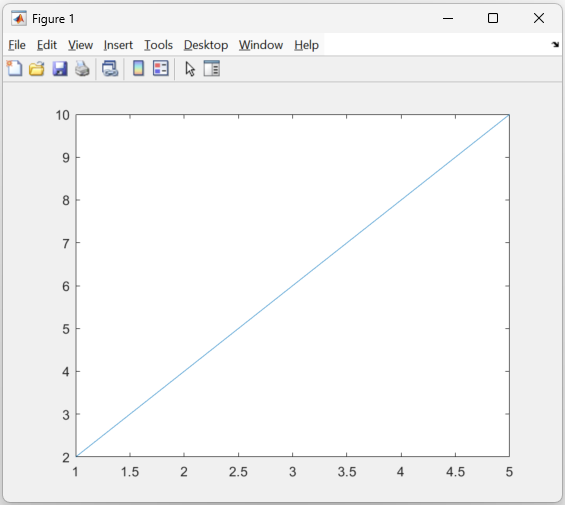
Basic Plot

Create a basic 2D line plot with the following variables

Instructor Note

Good place to demonstrate the interactivity of MATLAB figures. Show zooming, saving, etc.

MATLAB


x = [1 2 3 4 5];
y1 = [2 4 6 8 10];

plot(x,y1)

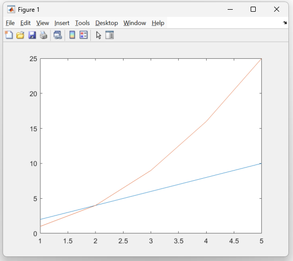
hold on

To add another line to the same plot we can use the hold on command, this will retain the current figure when adding new plots.

hold on

Create another vector variable called y2 with values 1, 4, 9, 16, 25

Plot x against y1 then x against y2 without hold on, what happens?
Plot x against y1, then hold on, then x against y2, what’s different?

Show me the solution

You should only see the y2 line, as the y1 figure was overwritten without hold on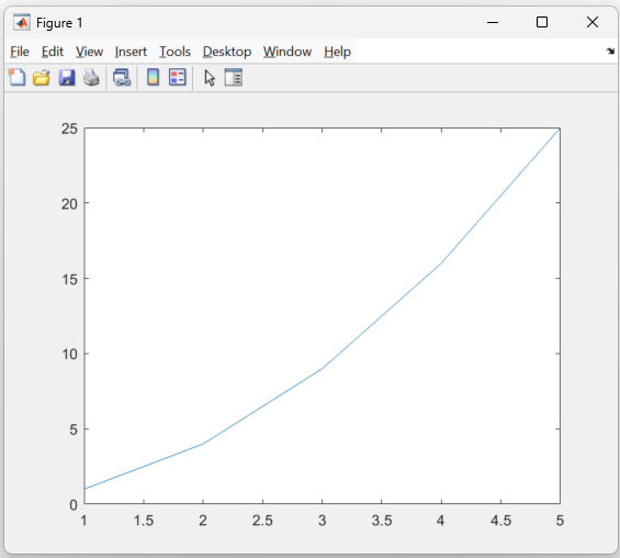
Now you should have both lines on the same plot

Line and Marker Styling

MATLAB offers a range of line colours and markers which can help distinguish lines or theme them.

Here are links to the line style and plot colour guides.

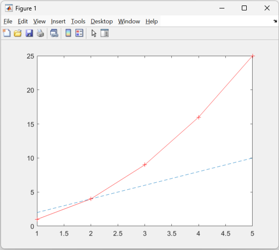
Styled plots

Close any currently open figures and use the guides above to plot the following lines:

Plot y1 against x with a dashed line
Plot y2 against x using a red solid line with plus markers

Show me the solution

MATLAB


plot(x,y1, '--')
hold on
plot(x,y2, '+-r')

Callout

There are many other 2D plot types available in MATLAB which mostly use a very similar syntax to plot, such as:

bar, histogram, scatter, heatmap and more. The full list can be found here

Figure Labelling

Titles, axis labels and legends are useful tools to make your plots more readable, and are essential to a plot if it is being added to a paper or journal.

MATLAB

title('Comparison of 2 lines')

xlabel('X Numbers')
ylabel('Y Numbers')

legend('Straight', 'Exponential')

3D Plotting

Here we are going to use a MATLAB function called peaks, which is a useful function for demonstrating 3D figures. It generates a matrix containing peaks obtained from a Gaussian distribution.

z = peaks(50);
surf(z)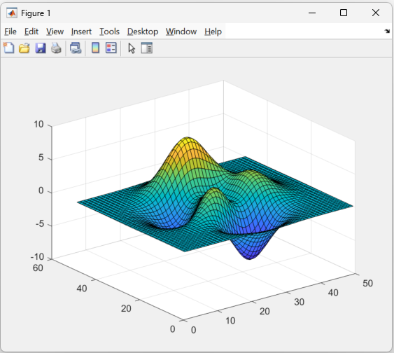

A screenshot of a MATLAB figure containing a 3D surface plot with peaks

Key Points

Figures in MATLAB are by default interactive
Hold on is needed to place multiple plots on the same figure
Label and title your plots for extra clarity

Content from Logic

Last updated on 2025-04-28 | Edit this page

Estimated time: 12 minutes

Overview

Questions

How can I make my code do different things when variables change?
How can I compare values in an array to other values?
How can I select subsets of my data depending on a comparison?

Objectives

Learn to use relational operators to compare values
Understand if and else statements to create conditional code
Learn some new tools and functions relating to logic

Relational Operators

Relational operators are used to compare the values in 2 arrays and returns a logical array.

Here are the most common logical operators in MATLAB:

MATLAB

data == 50 % Are any data points equal to 50?
data ~= 50 % Are any data points not equal to 50?
data > 50 % Are any data points greater than 50?
data < 50 % Are any data points less than 50?
data >= 50 % Are any data points greater than or equal to 50?
data <= 50 % Are any data points less than or equal to 50?

Here is an example of comparing two arrays:

MATLAB


a = [1 1 1 1];
b = [1 2 1 2];

a == b

OUTPUT

ans =

  1×4 logical array

   1   0   1   0

MATLAB Logic

MATLAB represents logical true and false statements with 1 and 0, where 1 is true and 0 is false

The returned logical array tells us that the first values were equal, the second not equal, etc.

If Statements

If statements allow us to execute different lines of code depending on a logical value.

MATLAB

c = 10

if c > 0
  disp('c is positive')
end

OUTPUT

c is positive

In this example, c > 0 is called the condition, disp('c is positive') is the code which will be executed if the condition is true, and every if statement in MATLAB should be terminated with an end

We can use some inbuilt functions such as any or all to test a condition across an entire array.

For example, we have a data set representing student marks called data, where each value is a mark out of 100, each row a student and each column a subject:

MATLAB

student_marks = round(100*rand(4,6));

We could test if any there any marks below or equal to 10 with the following code

MATLAB



if any(student_marks < 10)
  disp('Severe failing mark in dataset')
end

Challenge

Using the student_marks data above, display a sentence if any student achieves a first (70 or more) in the 3rd subject

Show me the solution

MATLAB


if any(student_marks(:,3) >= 70)
  disp('At least 1 student has achieved a first in subject 3')
end

if else elseif

Conditions can be chained together using the else and elseif terms. This allows for multiple different code blocks to be used depending on multiple conditions.

MATLAB

if all(student_marks(:,2) >= 70)
  disp('All students have a first in subject 2')
elseif any(student_marks(:,2) >= 70)
  disp('At least 1 student has a first in subject 2')
else
  disp('No students have a first in subject 2')
end

Logical Indexing

In the working with variables chapter, we looked at how we can index a variable with row and column numbers.

MATLAB

data = [1 3 5 7; 2 4 6 8];
data(2,4)

OUTPUT

Here we will look at indexing using logic arrays, which going back are the result of relational operators.

MATLAB

big_data = data >= 4 

data(big_data)

OUTPUT

First we create a logical array called big_data, which is the result of us looking for numbers in our data greater than or equal to 4.

We can then use this to index data, like slicing by index number, the result being only the part of data that is bigger than 4.

These two lines can be combined as well, avoiding the need to save the logical array as it’s own variable

MATLAB

data(data >= 4)

OUTPUT

logical not

A useful tool when handling logical arrays is the logical not, represented with the ~ symbol.

This operation inverts a logical array, which can be used to find values that don’t meet a condition.

MATLAB


big_data = data >= 4;
disp(big_data)
disp(~big_data)

OUTPUT

   0   0   1   1
   0   1   1   1

   1   1   0   0
   1   0   0   0

isnan

The final thing we will look at in this episode is the isnan function. This function returns a logical array containing true (1) where there is a NaN in the array. This could be used to replace the NaN values with a default value like 0, or combined with the logical not to only select non-nan data:

MATLAB

data = [2 4 NaN 8; 1 NaN 5 7];

data = data(~isnan(data))

OUTPUT

Key Points

The result of a relational operator is a logical array
if, elseif and else can be used to create powerful conditions
Logical arrays can be used to index variables

Content from Control

Last updated on 2025-04-28 | Edit this page

Estimated time: 12 minutes

Overview

Questions

What are the different types of loop?
How can you control loops to exit early or skip iterations?
How can you loop over multiple objects at the same time?

Objectives

Understand the main types of loop and when they should be used
Learn about loop controls such as break and continue

Loops in coding allow for blocks of code to be executed multiple times depending on some logic. This can save you from having redundant copy and pasted code, making your code shorter and easier to read.

There are two main loop types in MATLAB, for loops and while loops. A for loop repeats a specified number of times, a while loop repeats until a logical condition is met.

For Loops

For loops have the following syntax

for index = values
  code
end

values is typically a vector where the length will define the number of repetitions

index will be the current value of values for this iteration. In the exaple below,

MATLAB

A = 1:5;
for ii = A
  disp(ii)
end

``` OUTPUT
1
2
3
4
5

In this example our values is 1:5 which if you remember from indexing produces a vector [1 2 3 4 5]

So our for loop, loops 5 times, the first loop our index ii will be 1, then 2, etc.

Challenge

Create a for loop that sums the even numbers in the range 0 to 20.

Give me a hint

Try creating another variable called total equal to 0, for each iteration of the loop add the current index

Also think back to previous episodes where we covered indexes and counting in steps

Show me the solution

MATLAB

total = 0
for ii = 0:2:20
  total = total + ii;
end

While Loops

As previously mentioned, while loops will loop while a logical condition is being met.

MATLAB

ii = 0
while ii < 10
  ii = ii + 1;
end

Interestingly, as 1 is logic true in MATLAB, the following loop will run until cancelled or MATLAB runs out of resources

Cancel execution

While loops can get stuck in an infinite cycle, to stop this running without shutting MATLAB you can press Ctrl+C or on Mac Ctrl+Break

MATLAB

ii = 0
while 1
  ii = ii + 1;
end

While loops are useful when you don’t know how many iterations are needed. Some common use cases are:

Iterative Algorithms: Gradient-descent in machine learning, power series
Event driven: Continuously reading from a sensor, waiting for user input

Loop Controls

break and continue are statements that can be used to control behavior in a loop

The break statement immediately exits the loop it’s in, skipping any remaining iterations. Execution continues with the next statement after the loop.

MATLAB

for ii = 1:10
    if ii == 5
        break;
    end
    disp(ii);
end
disp('Loop finished');

OUTPUT

1
2
3
4
Loop finished

The continue statement skips the remaining code in the current iteration and jumps to the next iteration of the loop.

MATLAB

for ii = 1:8
    if mod(ii, 2) == 0 % Check for even numbers
        continue; 
    end
    disp(ii);
end

OUTPUT

Nested Loops

You may come across a situation when programming where you need to need to process every element of one dataset against every element of another. This scenario is often tackled using a nested loop, where you have one for loop inside of another.

This example multiplies each number from two ranges against each other, displaying the current iterators and the resulting product for each loop.

MATLAB

for ii=1:3
  for jj=10:10:30
    ii
    jj
    ii*jj
  end
end

Callout

Nested loops are powerful tools but avoid nesting unnecessarily. Code nested 3 or 4 loops deep can be hard to understand and read.

Key Points

Use for loops for when you know how many iterations to loop, while loops when you don’t
Break and continue allow you to exit or skip loops
Use indents to keep looped code clear